Introducing a large panel dataset of economy-wide real electricity prices and estimating long-run GDP and price elasticities of electricity demand for high- and middle-income panels

Increasing the share of energy services that are delivered via electricity is one of two challenges/strategies for mitigating climate change (decarbonizing electricity generation being the other). So, analyzing economy-wide electricity demand is an important research topic. But the availability of price data often constrains such energy demand analyses—particularly the study of demand in non-OECD countries.

Hence, we assemble a particularly large dataset of real economy-wide electricity prices (in 2015 US cents per kilowatt hour). This unbalanced electricity price data span 1978-2019 and include 107 countries. A key aspect of the price data is that it is a real price—as opposed to a real index. Thus, it is appropriate for cross-sectional analyses (in addition to panel analyses). Similarly, over-time averages could be compared across countries. An index, in contrast, is not meaningful cross-sectionally (e.g., it is 100 for all countries in the base-year). This short paper introduces the dataset, describes its construction (and its limitations), and displays some of the country series. Then it concludes with an example of the dataset’s usefulness—estimating economy-wide GDP and price elasticities for high- and middle-income panels. This example, suggests that estimating GDP elasticities without the consideration of prices may impart an upward omitted variable bias.

We begin with electricity prices for industry and residential households (in 2015 US cents per kilowatt hour and including taxes) from Enerdata’s Global Energy and CO₂ database.1 We then weight those two prices by their electricity final consumption (data from Enerdata as well).

For several countries, we extend this real weighted price via the International Energy Agency’s (IEA) real electricity price index for industry and households2 (which typically runs 1978-2019). For 17 OECD countries, a real electricity price index derived from Baade3 is used to extend those countries’ price series from 1978 to 1960. Following the standard procedure for splicing time series, our 1978 price level was extrapolated backward in time by the growth rates in electricity prices reported in the Baade analysis. This approach combined with the Baade data has been used to similarly extend price data in, for example, Adeyemi and Hunt4 and Liddle and Huntington.5 For five Asian economies, a real electricity price index derived from Pesaran et al.,6 which has price data from 1972-1992, was used to extend those economies price series. The Pesaran et al. data were used in a similar fashion in Liddle and Huntington.7 (The associated dataset indicates which observations have been extended and by which additional source.)

Agriculture and transport were not considered in constructing the price series. According to IEA data, agriculture and transport together account for less than five percent of electricity consumption in most countries.

Potentially, a greater concern is not including data from commercial use. Electricity in commercial buildings is substantial in most countries (representing, on average, 28% of electricity consumption according to IEA data); however, Enerdata does not report prices for commercial buildings. Commercial prices are typically between residential and industry prices and, usually, much closer to residential prices than industry. For example, in the US, commercial electricity prices ranged from 18% to 6 % lower than residential prices over 1990-2019 (data from Energy Information Administration). IEA has relative price data (residential, commercial, industry) for a few OECD and non-OECD countries. For most of these countries, residential prices are the highest, industry prices the lowest, and commercial prices on average are roughly the same as or within 20% of residential prices. For the countries where this was not the case, commercial prices tended to be the highest and residential prices the lowest. Correspondingly, for several of these latter countries (India, Nepal, Pakistan), commercial buildings comprised a relatively small share of total electricity consumption (10-15%), and for Iran, commercial prices were very similar to industry prices. Thus, we believe that the exclusion of commercial electricity prices on average should not bias the economy-wide price estimates.

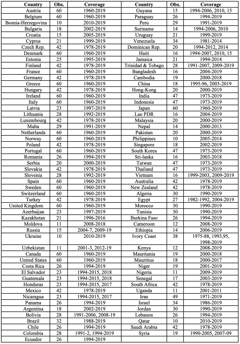
All told this real electricity price (unbalanced) dataset spans 1960-2019 and consists of the 107 countries for which there are at least 10 observations; 36 countries have at least 40 observations (with 17 of those having the full 60), and another 40 have at least 20 observations. Table 1 lists the country coverage.

We conclude the introduction of the data by displaying some of the price series. Figure 1 shows the real electricity prices (in 2015 US cents/kWh) for most European countries from 1960-2019. Two patterns stand out in Figure 1: (1) there has been a high degree of convergence in prices among European countries; and (2) electricity prices no longer follow the pattern of international oil prices.

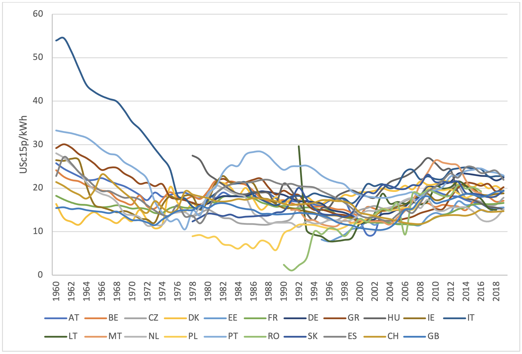
The international oil price tended to decline slightly during the 1960s, then rose through the 1970s because of Middle Eastern oil supply disruptions. After reaching a peak in 1982, oil prices declined and remained relatively low for more than two decades before rising beginning in 2004. By 2008, oil prices reached a level similar to their previous peak, but declined rapidly during 2014-2015 and have stayed relatively low since.

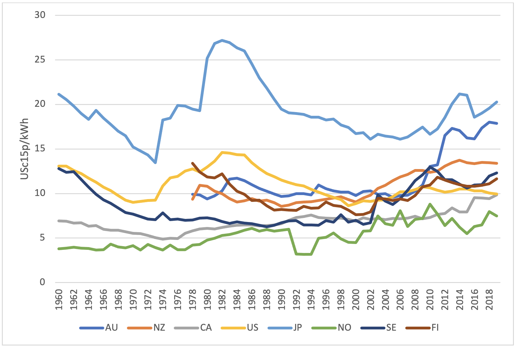
Figure 2 displays electricity prices for three Scandinavian countries (Finland, Norway, and Sweden) that have particularly low electricity prices because of the share of renewable energy (between 80% and 100% from renewable sources) and for several non-European OECD countries. Like those Scandinavian countries, Canada, New Zealand, US, and, until recently, Australia have had relatively low electricity prices. Electricity prices in Japan still appear to mimic international oil prices; whereas, this is no longer the case for US.

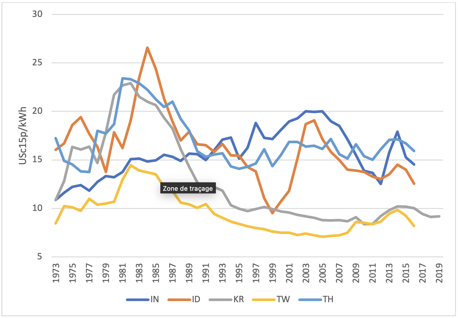
Lastly, Figure 3 contains the price paths for five rapidly growing Asian countries/economies. As above, local electricity prices have mostly broken from international oil prices, and electricity prices are particularly low for Korea and Chinese Taipei (two countries that have higher per capita electricity consumption than many European and other OECD countries).

An Example: Estimating Economy-wide GDP and Price Elasticities

As is standard in the energy demand literature, we estimate per capita electricity consumption as a function of per capita GDP (income) and electricity prices:
ln Electricity_it=α_i+β_i²ln GDP_it+β_i³ln price_it+ε_it  (1)

where t represents the time dimension and i the country dimension; α is a cross-sectional specific constant; the βs are cross-sectional specific coefficients to be estimated; and ε_it is the error term. It also is common to allow for the gradual adjustments—differences between short-run and long-run effects—to analyze a dynamic model:
ln Electricity_it=α_i+β_i¹ln Electricity_it-1+β_i²ln GDP_it+β_i³ln price_it+ε_it  (2)

For this dynamic, partial adjustment model, the long-run GDP and price elasticities, respectively, are:
 (3)

One also can consider more complex dynamics—i.e., additional lags of the GDP and price terms (see Liddle and Huntington 2020 for a detailed discussion of dynamic panel energy models). Because of data limitations in panel estimations, we limit ourselves to only one lag for GDP and price:
ln Electricity_it=α_i+β_i¹ln Electricity_it-1+β_i²ln GDP_it+β_i³ln price_it+β_i⁴ln GDP_it-1+β_i⁵ln price_it-1+ε_it (4)

Now, the long-run GDP and price elasticities are estimated via:

 (5)

In choosing an estimation method, there are several issues one must consider for this type of long, macro-panel data (for a more detailed discussion of each of these issues in the context of panel energy demand modeling, again, see Liddle and Huntington 2020). First, it is likely that elasticities will be different across countries. Hence, we use a mean group estimator (MG) that first estimates coefficients from cross-sectional specific regressions and then averages those estimated individual-country coefficients to arrive at panel coefficients. Two other well-known statistical issues for macro-panels are cross-sectional dependence and non-stationarity. Thus, we include in the regression cross-sectional averages of the dependent and independent variables (following the Pesaran 2006 Common Correlated Effects—CCE—approach) to account for cross-sectional dependence and help produce stationary residuals.

In addition to addressing cross-sectional dependence, these cross-sectional average terms represent unobserved common factors, e.g., technology. Also, CCE is robust to nonstationarity, cointegration, breaks, and serial correlation. However, the CCE estimator is not consistent in dynamic panels since the lagged dependent variable is not strictly exogenous; thus, the Dynamic Common Correlated Effects (DCCE) estimator of Chudik and Pesaran8 includes additional lags of the cross-sectional means to become consistent again.

One last statistical issue is that dynamic models estimated with panel data are subject to a downward bias, called the dynamic panel or Nickell bias (static models, naturally avoid this bias). Since the dynamic panel bias is on the order of 1/T (Nickell 1981), it can be mitigated by having several time observations. Beck and Katz (2009) claimed that with at least 20 time observations, bias correction is counter-productive; whereas, Judson and Owen (1999) were more conservative, recommending bias correction unless there are at least 30 time observations. Bruno (2005) determined that in unbalanced panels (i.e., like our panels), the bias declines with average cross-sectional size (i.e., the bias is not determined entirely by the shortest series).

We construct two unbalanced panels: one consisting of high-income countries and the other middle-income countries (according to World Bank classifications). So, we collect electricity consumption per capita data (in kWh per capita) and GDP per capita data (in constant 2010 US$ at PPP) from IEA. Ultimately, the only data constraint are the availability of the price data. The unbalanced high-income panel has 35 countries9 and spans 1960-2019. All of those countries have at least 21 years of price data, 17 have the full 60 years, and the average number of price observations is 48. The unbalanced middle-income panel has 34 countries10 and spans 1973-2018. All of those countries have at least 20 years of price data, four have the full 46 years, and the average number of price observations is 30.6. Thus, even according to the conservative rule of thumb of Judson and Owen, dynamic panel bias should be minimized at least.

Because of the lack of available price data for non-OECD countries, we know of no previous panel-based analyses of economy-wide electricity demand (that included both GDP and electricity prices) focusing on such countries. There have been a few such previous panel-based analyses that used OECD/EU data. Lee and Lee (2010) considered a panel of 25 OECD countries that spanned 1978-2004 and used a static model employing first-generation methods (i.e., methods that ignore potential cross-sectional dependence). Their GDP elasticity was significant and rather large at 1.08, but their price elasticity was very small and highly insignificant (-0.01). Lee and Chiu (2011) considered nearly the same panel, but used methods that allowed for nonlinearities and change over time (but still no consideration of cross-sectional dependence). Lee and Chiu found an average GDP elasticity of 0.36 and an insignificant price elasticity around -0.23. Recently, Arcabic et al. (2021) analyzed a sample of EU countries considering quarterly data over 2003-2018 and used a method that approximated smooth structural breaks with a Fourier function. For their preferred specification, they calculated an average long-run income elasticity of around 0.3 and an average long-run price elasticity of less than -0.04.

Our long-run elasticity results are displayed in Table 2. For the high-income panel, we show results from all three models (i.e., Equations 1, 2, and 4). For the middle-income panel, we do not show the results from the model using Equation 4 since the hypothesis that the one period lags of GDP and Price (i.e., β⁴ and β⁵ from Equation 4) were jointly equal to zero could not be rejected.

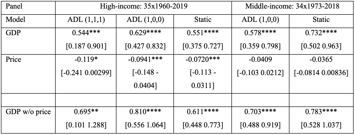
The GDP elasticities are all highly significant and similar both among the different models and for the high- and middle-income panels (particularly so when the dynamic model is considered). The GDP elasticities suggest that GDP will grow faster than per capita electricity consumption. Also, all of the GDP elasticity estimates are significantly below unity (one is not contained in their 95% confidence intervals). Thus, electricity intensity (electricity consumption/GDP) will decline with economic growth. The price elasticities are all small and negative. They are, however, statistically significant for the high-income panel.

Comparing our high-income panel results to the previous analyses, our price elasticity estimates (while significant) are between those of Lee and Chiu and Arcabic et al. While our GDP elasticity is larger than both of Lee and Chiu and Arcabic et al., it is substantially smaller than that of Lee and Lee. It is important to note that our time span is considerably larger than the previous three papers. Furthermore, while Lee and Chiu and Arcabic et al. allowed for some flexibility in terms of nonlinearities and temporal heterogeneity, neither of those papers adjusted for cross-sectional dependence.

Lastly, in considering the results from the models run without price information, we can draw several important conclusions. Each of the GDP elasticity estimates without prices considered are larger than the corresponding estimate when prices were considered; most of the estimates without prices were less precise (their confidence intervals were larger) than estimates with prices, and most of the estimates without prices were not statistically different from unity (one was within the confidence interval). These differences occurred even though the price elasticities themselves were very small, and in the case of the middle-income panel statistically insignificant. Thus, including prices in panel electricity demand estimations may improve the precision of the GDP elasticity estimates, and not including prices can lead to (an apparent upward) omitted variable bias in those GDP elasticity estimates. Thus, this rather large database of economy-wide electricity real prices should prove valuable to future analyses.  

• 1. Enerdata, “Global Energy & CO2 database”. Url : https://www.enerdata.net/research/energy-market-data-co2-emissions-data… (accessed 11/11/2021).
• 2. OECD iLibrary, “IEA Energy Prices and Taxes Statistics”. Url: https://www.oecd-ilibrary.org/energy/data/end-use-prices/indices-of-ene… (accessed 11/11/2021)
• 3. P. Baade, International Energy Evaluation System, International Energy Prices 1955-1980 (Service Report, U.S. Department of Energy, 1981/21).
• 4. O. Adeyemi, L. Hunt, “Modelling OECD Industrial Energy Demand: Asymmetric Price Responses and Energy-saving Technical Change”, Energy Economics, vol. 29, no 4, 2007.
• 5. B. Liddle, H. Huntington, “Revisiting the Income Elasticity of Energy Consumption: A Heterogeneous, Common Factor, Dynamic OECD & non-OECD Country Panel Analysis”, The Energy Journal, vol. 41, no 3, 2020.
• 6. H. Pesaran et al., Energy Demand in Asian Developing Economies (Oxford: Oxford University Press for the World Bank and the Oxford Institute for Energy Studies, 1998).
• 7. B. Liddle, H. Huntington, “Revisiting the Income Elasticity of Energy Consumption: A Heterogeneous, Common Factor, Dynamic OECD & non-OECD Country Panel Analysis”, The Energy Journal, vol. 41, no 3, 2020.
• 8. A. Chudik, H. Pesaran, “Common correlated effects estimation of heterogeneous dynamic panel data models with weakly exogenous regressions”, Journal of Econometrics, vol. 188, no 2, 2015, 393-420. The Dynamic Common Correlated Effects estimator is implemented by Stata command xtmg—which was developed by Markus Eberhardt.
• 9. Those countries are: Australia, Austria, Belgium, Canada, Chinese Taipei, Cyprus, Czech Republic, Denmark, Estonia, Finland, France, Germany, Greece, Hungary, Israel, Ireland, Italy, Japan, Korea, Latvia, Lithuania, Luxembourg, Malta, Netherlands, New Zealand, Norway, Poland, Portugal, Slovakia, Slovenia, Spain, Sweden, Switzerland, United Kingdom, and USA.
• 10. Those countries are: Algeria, Azerbaijan, Bolivia, Brazil, Chile, Columbia, Costa Rica, Ecuador, El Salvador, Guatemala, Honduras, India, Indonesia, Iran, Ivory Coast, Jamaica, Jordan, Kazakhstan, Lebanon, Morocco, Mexico, Nicaragua, Panama, Paraguay, Peru, Romania, Saudi Arabia, South Africa, Thailand, Trinidad and Tobago, Tunisia, Turkey, Uruguay, and Venezuela.